Examples
import beautifulplots as bp
import matplotlib.pyplot as plt
import pandas as pd
import seaborn as sns
Barplot
# reset plot defaults for these examples
import matplotlib as mpl
mpl.rcParams.update(mpl.rcParamsDefault)
# Data and Dataframe
print('Data:Product Category Sales by Store')
barplot_data = { 'category':['groceries','groceries','groceries', 'hardware','hardware','hardware','hobbies','hobbies','hobbies'] ,
'sales':[ 900, 600,500, 500,300,200,400,400,200], 'store':['Store-A','Store-B','Store-C','Store-A','Store-B','Store-C','Store-A','Store-B','Store-C'] }
df = pd.DataFrame(barplot_data)
# unit sales by category ... assume some average sale price per category
def unit_sales(row):
units = 0
if row['category'] == 'groceries': units = row['sales']/5
elif row['category'] == 'hardware': units = row['sales']/10
elif row['category'] == 'hobbies': units = row['sales']/20
return units
df['units']= df.apply(lambda row: unit_sales(row),axis=1)
display(df)
# Plots
# Example 1a
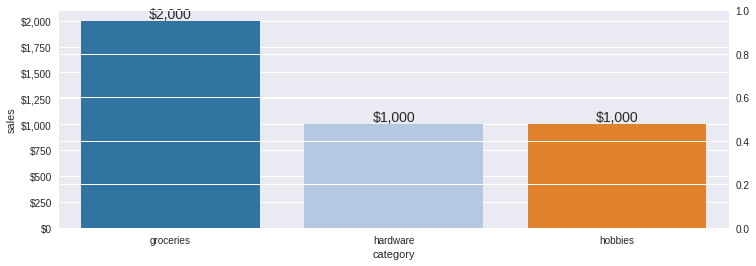
bp.barplot(df,'category','sales', palette='tab20',
title='1a. Beautifulplots barplot, Sales All Stores by Product Category, secondary y-axis', figsize=(12,4),
bardatalabels=True, bardataformat=",.0f", barcurrency="$", ylims = (0.1,2200), estimator2=sum,
y2='units',ylims2=(0,450),y2label='units', color2='black',marker2="o", y2axisformat=".0f")
# Example 1b
bp.barplot(df,'category','sales',hue='store', palette='tab20',
title='1b. Beautifulplots barplot, Sales by Store by Product Category, vertical', figsize=(12,4),
bardatalabels=True, barcurrency="$", bardataformat=",.0f",
ylims = (0.1,1000))
# Example 1c
bp.barplot(df,'category','sales',hue='store', palette='tab20',
title='1c. Beautifulplots barplot, Sales by Store by Product Category, horizontal', figsize=(12,8),
bardatalabels=True, bardataformat=".0f", barcurrency="$", barorientation='h',
xlims = (0.1,1000), legendloc="lower right")
Data:Product Category Sales by Store
| category | sales | store | units | |
|---|---|---|---|---|
| 0 | groceries | 900 | Store-A | 180.0 |
| 1 | groceries | 600 | Store-B | 120.0 |
| 2 | groceries | 500 | Store-C | 100.0 |
| 3 | hardware | 500 | Store-A | 50.0 |
| 4 | hardware | 300 | Store-B | 30.0 |
| 5 | hardware | 200 | Store-C | 20.0 |
| 6 | hobbies | 400 | Store-A | 20.0 |
| 7 | hobbies | 400 | Store-B | 20.0 |
| 8 | hobbies | 200 | Store-C | 10.0 |
---------------------------------------------------------------------------
NameError                                 Traceback (most recent call last)
Input In [2], in <cell line: 26>()
     19 display(df)
     23 # Plots
     24
     25 # Example 1a
---> 26 bp.barplot(df,'category','sales', palette='tab20',
     27                    title='1a. Beautifulplots barplot, Sales All Stores by Product Category, secondary y-axis', figsize=(12,4),
     28                    bardatalabels=True, bardataformat=",.0f", barcurrency="$", ylims = (0.1,2200), estimator2=sum,
     29                    y2='units',ylims2=(0,450),y2label='units', color2='black',marker2="o", y2axisformat=".0f")
     31 # Example 1b
     32 bp.barplot(df,'category','sales',hue='store', palette='tab20',
     33                    title='1b. Beautifulplots barplot, Sales by Store by Product Category, vertical', figsize=(12,4),
     34                    bardatalabels=True, barcurrency="$", bardataformat=",.0f",
     35                    ylims = (0.1,1000))

File ~/checkouts/readthedocs.org/user_builds/beautifulplots/envs/stable/lib/python3.8/site-packages/beautifulplots/barplot.py:127, in barplot(df, bar_columns, bar_values, barcurrency, barorientation, bardataformat, y2, estimator, estimator2, ax, bardatalabels, test_mode, bardatafontsize, **kwargs)
    122     if not isinstance(marker2,list): marker2 =[marker2]
    124 _ax2 = _ax.twinx()
--> 127 for _y2,_marker2 in zip(y2_list,marker2):
    128     if plot_options['palette2'] !=None:
    129         g = sns.lineplot(data=df,x=x, y =_y2, hue=hue, palette=palette2,  ax=_ax2, label=_y2,
    130                          alpha = alpha2,ci = ci2, marker=_marker2, estimator=estimator2,
    131                          markers=markers2, style=style2)

NameError: name 'y2_list' is not defined
Lineplot, Stock Market S&P 500
# reset plot defaults for these examples
import matplotlib as mpl
import datetime as dt
mpl.rcParams.update(mpl.rcParamsDefault) # reset plot/figure parameters
# Data
sp500_file = '../data/GSPC_1950-1-3_to_2022-6-8.csv'
df_sp500 = pd.read_csv(sp500_file,index_col=0,parse_dates=True)
display(df_sp500.head())
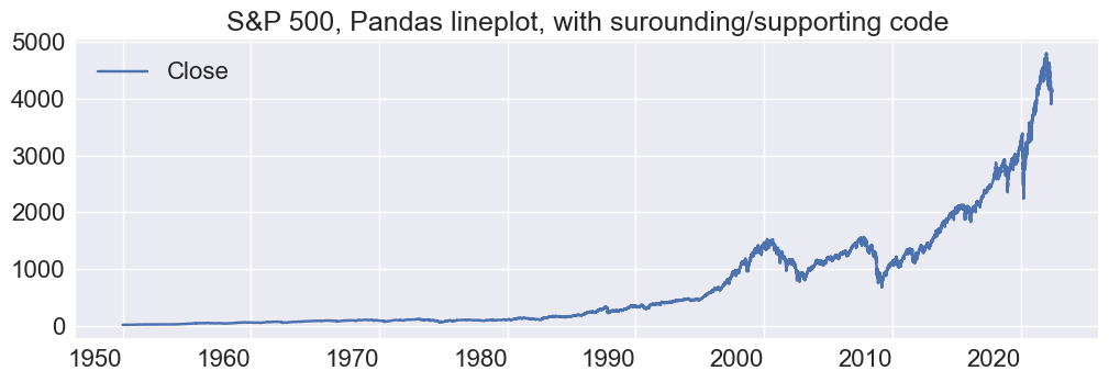
# Pandas Plot ... use beutifulplots plot_defualts and set_axisparams for improving pandas graph
print('Pandas lineplot')
plt.style.use('seaborn')
fig,ax = plt.subplots(nrows=1,ncols=1,figsize=(12,4))
plot_options = bp.plot_defaults()
plot_options['title']="S&P 500, Pandas lineplot, with surounding/supporting code"
g=df_sp500.plot(y='Close',ax=ax) # note, it handles date index well
bp.set_axisparams(plot_options,ax,g)
plt.show()
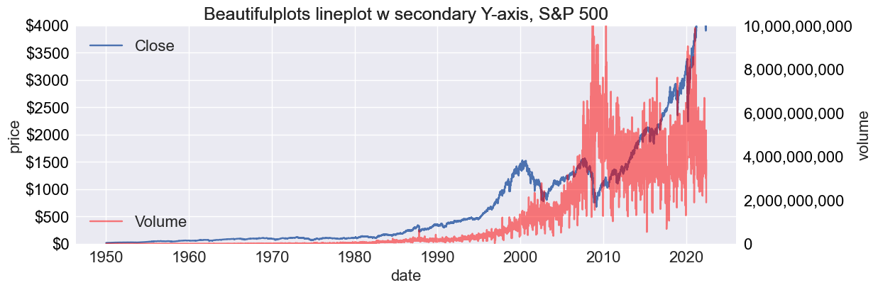
# reset index ... Seaborn and thus beautifulpltos requires x-axis to be a column
df = df_sp500.reset_index()
display(df)
# bp lineplot
bp.lineplot(df,x='Date' , y=['Close','Open'], y2='Volume',yaxisformat=".0f",ycurrency="$", y2axisformat=",.0f",
ylims=(0,4000), ylims2=(0,10*1e9), legend_loc2 = "lower left", color2='red', marker="o",
figsize=[12,4],yaxis_currency=True, legend=True, ylabel = "price", y2label="volume", xlabel="date",
ytick_format=".0f", title="Beautifulplots lineplot w secondary Y-axis, S&P 500")
| Close | High | Low | Open | Volume | Adj Close | |
|---|---|---|---|---|---|---|
| Date | ||||||
| 1950-01-03 | 16.66 | 16.66 | 16.66 | 16.66 | 1260000.0 | NaN |
| 1950-01-04 | 16.85 | 16.85 | 16.85 | 16.85 | 1890000.0 | NaN |
| 1950-01-05 | 16.93 | 16.93 | 16.93 | 16.93 | 2550000.0 | NaN |
| 1950-01-06 | 16.98 | 16.98 | 16.98 | 16.98 | 2010000.0 | NaN |
| 1950-01-09 | 17.08 | 17.08 | 17.08 | 17.08 | 2520000.0 | NaN |
Pandas lineplot
| Date | Close | High | Low | Open | Volume | Adj Close | |
|---|---|---|---|---|---|---|---|
| 0 | 1950-01-03 | 16.660000 | 16.660000 | 16.660000 | 16.660000 | 1.260000e+06 | NaN |
| 1 | 1950-01-04 | 16.850000 | 16.850000 | 16.850000 | 16.850000 | 1.890000e+06 | NaN |
| 2 | 1950-01-05 | 16.930000 | 16.930000 | 16.930000 | 16.930000 | 2.550000e+06 | NaN |
| 3 | 1950-01-06 | 16.980000 | 16.980000 | 16.980000 | 16.980000 | 2.010000e+06 | NaN |
| 4 | 1950-01-09 | 17.080000 | 17.080000 | 17.080000 | 17.080000 | 2.520000e+06 | NaN |
| ... | ... | ... | ... | ... | ... | ... | ... |
| 18158 | 2022-06-02 | 4176.819824 | 4177.509766 | 4074.370117 | 4095.409912 | 3.604930e+09 | 4176.819824 |
| 18159 | 2022-06-03 | 4108.540039 | 4142.669922 | 4098.669922 | 4137.569824 | 3.107080e+09 | 4108.540039 |
| 18160 | 2022-06-06 | 4121.430176 | 4168.779785 | 4109.180176 | 4134.720215 | 3.852050e+09 | 4121.430176 |
| 18161 | 2022-06-07 | 4160.680176 | 4164.859863 | 4080.189941 | 4096.470215 | 3.476470e+09 | 4160.680176 |
| 18162 | 2022-06-08 | 4115.770020 | 4160.140137 | 4107.200195 | 4147.120117 | 1.888845e+09 | 4115.770020 |
18163 rows × 7 columns
help - plot_defaults, barplot, lineplot
help plot_defaults
help(bp.plot_defaults)
Help on function plot_defaults in module beautifulplots.beautifulplots:

plot_defaults()
    Dictionary of plot parameters. Each parameter coresponds and corresponding value.
    See also get_plot_options for extracting plot options from **kwargs.

    **Axis - x, y, and plot area parameters**

    Args:
        df (DataFrame): The input DataFrame containing colums corresponding to bar values and columns.

        title (String): corresponds to the axis title. default = ''

        titlefontsize: font size of the axis title, default = 18

        legend_loc(String): Matplotlib legend location, for example, upper right , default = "best".

        legend_loc2 (String): Secondary axis legend location, for example, upper right , default = best.

        xlims: (xmin, xmax), minimum and maximum x-values of the axis. default = None, in which case the min and max are set automatically by matplotlib.

        ylims: (ymin,ymax), minimum and maximum y-values of the axis. default = None, in which case the min and max are set automatically by matplotlib.

        ylims2: (ymin,ymax), minimum and maximum y-values of the secondary axis. default = None, in which case the min and max are set automatically by matplotlib.

        xlabelfontsize: default = 16

        xticklabelsize: default = 16

        xtickfontsize: default = 16

        xtickrotation: default = 0

        ylabelfontsize: ylabel font size, default = 16

        ytickfontsize: xtick label font size, default = 16

        ytickrotation:  Rotation of the xtick label, default = 0

        legendfontsize: legend font size, default = 16

        xlabel (String): xlabel title, default = ''

        ylabel (String):  ylable title, default = ''

    **Line, Scatter Plots**

    Args:

        marker: Matplotlib line markers. default = None (Matplotlib default).

        marker2: Secondary axis, Matplotlib line marker. default = None (Matplotlib default).

        yaxis_currency (Boolean): Boolean default = False.

        ytick_format (String): String default = None (Matplotlib default).

        alpha (fraction): Trasnparancy (opacity), default = None (not transparent)

        alpha2 (fraction): Secondary axis, default = 0.5, 50% opacity

        legend_labels (list): Overide default legend labels. default = None (do not override)

        estimator: seaborn barplot summary estimator, default = sum

        estimator2: secondary axis, seaborn barplot summary estimator, default = sum

        color: default = None, indicateing Matplolib default (Matplotlib default)

        color2: secondary axis line, bar or color. defualt = None (Matplotlib default)

        palette: colormap, default = None

        palette2: colormap, default = None, secondary y axis.

        hue: dimension value for corresponding Seaborn graphs, default = None.

        ci: Seaborn confidence interval parameter: float, sd, or None

        ci2: Seaborn confidence interval parameter second y axis: float, sd, or None

    **Plots and subplots**

    Parameters corresponding to the plot or subplot characteristics. They are used when matplot_helpers
    functions create the plot figure and axis, otherewise, these parameters do not affect the plot.

    Args:

        plotstyle (String): matplotlib plotstyle

        figsize: total size (height, width) in inches of the figure, including total plotting area of all subplots and spacing

        wspace: width space (horizontal) between subplots, default wspace = 0.2

        hspace: height space (vertical) between subplots, default hspace = 0.2

        legendloc: default=best

    **Returns**

        Dictionary: {parameter1:value1, parameter2:value2, ... }.
        Pairs of plat parameters and corresponding values.
help barplot
help(bp.barplot)
Help on function barplot in module beautifulplots.barplot:

barplot(df, bar_columns, bar_values, barcurrency=None, barorientation='v', bardataformat='1.2f', y2=None, y2axisformat='1.2f', y2currency=None, estimator=<built-in function sum>, estimator2=None, ax=None, bardatalabels=False, test_mode=False, bardatafontsize=14, **kwargs)
    Bar plot function designed for ease of use and aesthetics.
    The underlying barplot is ased on the Seaborn with additions, such as secondary axis, data labels,
    and improved default parameters. Refer to beautifulplots plot_defaults for a complete list of options.

    Args:
        df (DataFrame): The input DataFrame containing colums corresponding to bar_plot values ("bar_values") and column names (see examples in documentation)

        bar_columns: Datafrae columns corresponding to bar column names

        bar_values: Dataframe column corresponding to bar column values

        ax (axis): matplotlib axis (optional), default = None. If axis is None, then create a matplolib figure, axis to host the barplot

        color: Matplotlib compatabile color name as text or RGB values, for example,  color = [51/235,125/235,183/235].

        palette: Matplotlib compatible color palette name, for example, "tab20"

        hue: Name of hue dimension variable (i.e., DataFrame column name)

        ci: Seaborn confidence interval parameter: float, sd, or None, default = None

        barorientation: default = v (vertical), or h (horizontal)

        barcurrency: default = False (bar values do not represent currency). True (bar values represent currency, append $ to the value)

        bardatalabels (Boolean): default = False (data labels not included)

        additional options:  see kale.plot_defaults for additional input variables.


    Returns:
        returns True if processing completes succesfully (without errors).
help lineplot
help(bp.lineplot)
Help on function lineplot in module beautifulplots.lineplot:

lineplot(df, x, y, yaxisformat='1.2f', ycurrency=None, y2=None, y2axisformat='1.2f', y2currency=None, ax=None, test_mode=False, estimator=None, estimator2=None, **kwargs)
    Lineplot function designed for ease of use and aesthetics. Based on the
    Seaborn lineplot function with improvements, such as secondary axis, ease of use, and
    improved default parameters. Refer to beautiful plot_defauts for full list of options.

    Args:
        df (Dataframe): The input DataFrame containing colums corresponding to x and y

        x: Dataframe column corresponding to the lineplot x-axis
            aldfsd;lfj

        y: Dolumn or list of columns corresponding to the lineplot y-axis

        y2: Column or list of columns correspondng to the secondary axis, default = None

    Returns:
        returns None if processing completes succesfully (without errors).